Paul Michael Kielstra

A tensor is a multidimensional array. A vector is a \(1\)-tensor; a matrix is a \(2\)-tensor. \(3\)-tensors, \(4\)-tensors, and so on also exist, and we treat them very similarly. If \(v\) is a vector, we might use \(v_i\) to refer to the \(i\)-th element. If \(A\) is a matrix, we might consider elements \(A_{ij}\). For higher-dimensional tensors, we just add more indices: \(T_{ijkl}\) refers to a specific element of the \(4\)-tensor \(T\).

The fundamental operation of matrix-matrix and matrix-vector pairs is multiplication. This boils down to a sum of products: the \(i\)-th element of the matrix-vector product \(Av\) is \(\sum_{j}A_{ij}v_{j}\). Since matrices and vectors have at most two dimensions, it’s easy to note down complicated strings of matrix and vector multiplications.

With tensors, however, writing out multiplications (or, in the more general language preferred for this more general setting, contractions) can be much more difficult. Consider the \(4\)-tensor \(Q\) given by multiplying the \(4\)-tensor \(T\) by the matrix \(A\) along each of its four dimensions. The elements of \(Q\) are given by \(Q_{pqrs}=\sum_{ijkl}T_{ijkl}A_{ip}A_{jq}A_{kr}A_{ls}\). And if that’s not already enough of a hassle, imagine if you were multiplying by different matrices along each dimension, or if you wanted to add in more tensors, or…

The solution is to give up on using \(\sum\) notation and instead display the tensors, and their connections, graphically. This is easier than it sounds. Here are a vector and a matrix, displayed as tensor network diagrams:

The dots, or nodes, represent tensors, and the lines, or edges, represent axes. The vector is one-dimensional, so it has one edge coming out of it. The matrix is two-dimensional, so it has two edges.

When you have one edge that connects two tensors, that means that you sum over that edge. This is a right-side vector-matrix multiplication, with \(j\)-th element given by \(\sum_{i}v_{i} A_{ij}\):

You’ll note that it has exactly one edge that’s only connected to one tensor. We say that such edges are dangling, and, in this case, we shouldn’t be surprised: the result of a vector-matrix product is a vector, so we should expect it to have one dimension, and each dangling edge represents a dimension.

Our giant four-way multiplication for \(Q\) now looks like this:

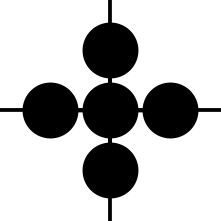
(Here, I haven’t labeled the nodes or the edges. Of course, you’re welcome to label them in your own diagrams.)

It should by now be obvious how useful tensor network diagrams can be for representing complicated tensor operations. To really prove their usefulness, though, I’ll leave you with my all-time favorite tensor network. First of all, consider what the following tensor network represents. (I would encourage you not to read further until you have at least a vague idea.)

Did you get it? It’s a matrix trace. The node has two edges coming out of it, so it’s a \(2\)-tensor, or a matrix, and we use the same index for both of those edges and sum over them, giving \(\sum_i A_{ii}\). This is exactly the trace of that matrix. (The tensor network doesn’t have any dangling edges at all, which is what we would expect: the trace of a matrix is a scalar, and so it has no dimensions.)

It’s occasionally useful to compute the trace of a matrix product \(AB\). Now, we can either work this out by algebra-bashing, or we can just draw the tensor network diagram for it:

Convince yourself first that this is the correct diagram. All I did to produce it was to substitute the diagram for a matrix-matrix multiplication, which you should draw out yourself, into the diagram for a trace. Now, let’s determine what formula this diagram is suggesting. It’s got two matrices, which we’ll call \(A\) and \(B\). It’s got two edges this time, both connecting \(A\) and \(B\). We’ll label the shorter edge \(i\) and the longer one \(j\). Then we just have to read off the formula \(\sum_{i, j}A_{ij}B_{ji}\). That’s our matrix product trace!