Paul Michael Kielstra

Let \(f\) be a function that you want to interpolate on the interval \([0, 1]\). Let \(k\) be some number of points. Say you know the values of \(f_i=f(i/k)\) for \(i=0, \dots, k-1\). If you knew that \(f\) were periodic with period \(1\), or in general if you knew that \(f\) decomposed into a sum of sinusoids with low frequencies, how might you leverage that knowledge to estimate \(f_{i+1/2}=f((i+1/2)/k)\)? (I’m assuming that the interpolation you have in mind exactly doubles the density of the grid. If you want to interpolate even more points, just repeat your procedure.)

Our assumptions on \(f\) boil down to “It’s a good idea to take a discrete Fourier transform here.” If we do that, we can reduce \(f\) to its component frequencies. Then, we can zero-pad the vector to increase the size of the frequency domain, do an inverse DFT to get back to a time domain, and we should be good to go.

(The inverse DFT formula contains a normalization term that divides by the number of points, so doubling the number of points in Fourier space will cut the magnitude of our function in half once the process is over. To correct this, we just have to multiply by \(2\).)

import numpy as np
import matplotlib.pyplot as plt

initial_N = 32
initial_sample_grid = np.linspace(0, 1, initial_N + 1)[:-1] # Remove final element because f(0)=f(1)
final_sample_grid = np.linspace(0, 1, 2 * initial_N + 1)[:-1]

def f(x):
    return np.cos(2 * np.pi * x) + 0.5 * np.sin(2 * np.pi * x)

f_values = f(initial_sample_grid)
f_transformed = np.fft.fft(f_values) # NumPy built-in FFT
f_zero_padded = np.concatenate((f_transformed, np.zeros(initial_N))) # [f1, f2, ..., fN, 0, ..., 0]
f_interpolated = 2 * np.fft.ifft(f_zero_padded)

plt.plot(final_sample_grid, f(final_sample_grid), label="True")
plt.plot(final_sample_grid, f_interpolated, label="Interpolated")
plt.legend()
plt.show()

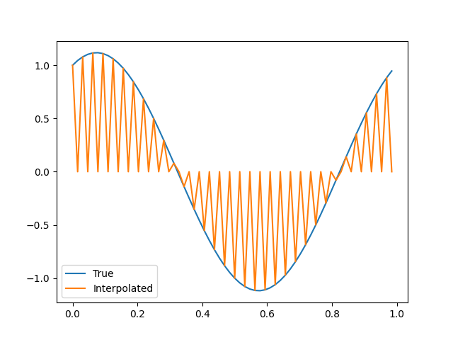
Oh dear.

Let’s not sell ourselves short: this is an interpolation. It successfully matches the value of \(f\) at all the data points we’ve given it. The problem, specifically, is that it introduces very high frequencies – frequencies, in particular, that could not be resolved on the original grid on which we sampled \(f\). Usually, we prefer our interpolations to be more conservative about these frequencies. We’re going to have to do something different.

To see exactly what, let’s take a look at the derivation of the DFT. Usually, we think of it in these terms:

But this is just a rewriting (using the fact \(e^{-2 \pi i} = 1\)) of the form

Here, the right-hand side is the actual Fourier transform, treating \(x\) as a continuous function, and the left-hand side is the discretization which focuses on the modes with lowest frequency. This is logical: those modes can be resolved on a sparse grid, while higher frequencies will require denser grids. In short, the discrete Fourier transform as usually implemented is “wrapped around” halfway. Rather than thinking of the lowest frequencies as being at the start or end of the vector we pass in, we should think of them as being in the middle.

This tells us why we’re introducing so many high frequencies into our interpolation. When we zero-pad on the right, we’re creating a vector with all the non-zero elements to the left of the midpoint and all the zeros to the right. This means we’ve got non-zero elements quite far away from the midpoint, and that means we’re going to get quite high frequencies. (We’re also going to get complex results, rather than purely real ones, since our frequencies with negative values of \(k\) have no corresponding positive values of \(k\) to cancel out the imaginary part. In fact, if you run the code, you should get an error complaining about discarding the imaginary part when you make the plot.)

With that in mind, it’s clear what we have to do. We need to add zeros where they correspond to high frequencies. In “standard” Fourier space, that’s far away from the midpoint, but, in wrapped-around Fourier space, it’s more complicated. The wrap-around takes vectors that look like

and spits out vectors that look like

The vector is cut in half and the first half is reversed and then put after the second.

If we pad our original vector with zeros on both sides, cut the result in half, reverse the first half of that, and put it after the second, we see that both the blocks of zeros wind up on the inside, thus:

This is actually really easy to get from our original wrapped-around vector. All we have to do is stick a bunch of zeros in the middle. That’s a one-line alteration to our code from earlier, which gives us the following:

import numpy as np
import matplotlib.pyplot as plt

initial_N = 32
initial_sample_grid = np.linspace(0, 1, initial_N + 1)[:-1] # Remove final element because f(0)=f(1)
final_sample_grid = np.linspace(0, 1, 2 * initial_N + 1)[:-1]

def f(x):
    return np.cos(2 * np.pi * x) + 0.5 * np.sin(2 * np.pi * x)

f_values = f(initial_sample_grid)
f_transformed = np.fft.fft(f_values) # NumPy built-in FFT
f_zero_padded = np.concatenate((f_transformed[:initial_N//2], np.zeros(initial_N), f_transformed[initial_N//2:])) # <-- CHANGE HERE
f_interpolated = 2 * np.fft.ifft(f_zero_padded)

plt.plot(final_sample_grid, f(final_sample_grid), label="True")
plt.plot(final_sample_grid, f_interpolated, label="Interpolated")
plt.legend()
plt.show()

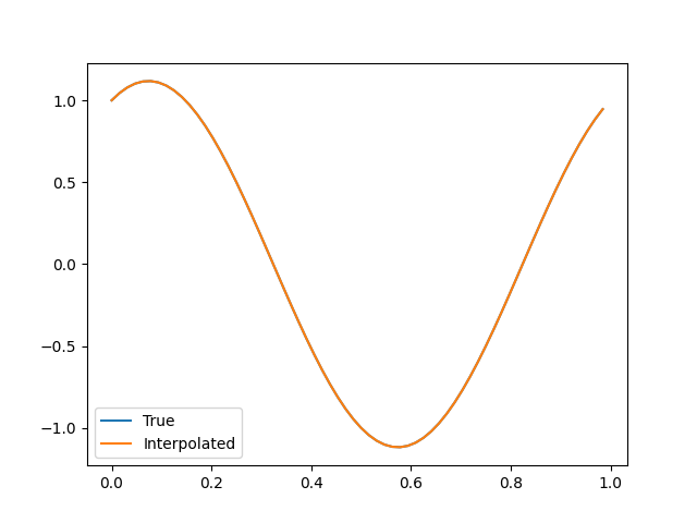
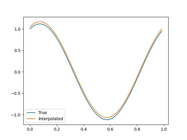
Much better. Here’s the result with the approximated value shifted by \(0.05\), so you can tell that this is actually working and not some sort of glitch:

The moral of the story: the DFT is not entirely a direct analogue of the continuous Fourier transform!

I found a few publications and articles helpful in writing this post:

• Fourier interpolation - Dan MacKinlay

• How to Interpolate in the Time-Domain by Zero-Padding in the Frequency Domain - Rick Lyons

• This Signal Processing Stack Exchange answer

• Interpolation Using the Discrete Fourier Transform - Gary Gramlich