Paul Michael Kielstra

Let \(f : \mathbb{R} \rightarrow \mathbb{R}\) be a periodic function with period \(2\). Then, for parameters \(a\) and \(b\), we define the Weierstrass sum to be the function \[W_{a,b}[f](x)=\sum_{n=0}^\infty a^n f(b^n x).\] In order for the sum to converge, we assume that \(0 < a < 1\); in order for the resulting function to have a fractal shape, we take \(b\) to be a positive odd integer.

The original motivation for this construction was to develop a function that was continuous everywhere but differentiable nowhere. This can be done by taking, for example, \(f(x)=\cos(\pi x)\) and choosing \(a\) and \(b\) such that \(ab>1+\frac{3}{2}\pi\). Continuous functions without any smoothness requirement are a natural fit for modeling by a quantized tensor train (QTT), and in fact \(W_{a,b}[f]\) can be written efficiently in this form for a great many \(f\)s.

Preliminaries

Let \(T \in \mathbb{R}^{d_1 \times \cdots \times d_n}\) be a tensor. A tensor train, or TT, representation of \(T\) is a sequence of \(3\)-tensors, or cores, \(A_1, \dots, A_n\) such that \[T(i_1,\dots,i_n) = \sum_{p_0,\dots,p_n}A_1(p_0, i_1, p_1)A_2(p_1, i_2, p_2)\cdots A_n(p_{n-1}, i_n, p_n).\] The first and third dimensions of each \(A_i\) are called the internal dimensions, while the second is the external dimension. The maximum internal dimension of a TT is its rank. The specific construction is beyond the scope of this post, but TTs can be added, producing the same result as adding the original tensors element-wise. The internal dimensions of the output TT are the sums of the relevant internal dimensions of the input TTs.

We can represent a vector with \(b^L\) elements by first reshaping that vector into a \(b \times \cdots \times b\) \(L\)-tensor and then representing that tensor as a TT. If we specifically do this to represent the values of a function on an interval, sampled at \(b^L\) equidistant points, we call the result a quantized tensor train, or QTT. Most definitions of QTTs specify \(b=2\); we will not be doing this. In fact, in this case, we are not overloading \(b\) at all. Throughout our construction, this value, the “base” of our QTT, will be the same as the \(b\) in the Weierstrass sum we wish to evaluate. (Note that this does restrict us to taking \(b\) to be a positive integer.)

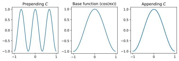
Let us first establish two preliminary constructions. Let \(C \in \mathbb{R}^{1 \times b \times 1}\) be a core with every entry equal to \(1\). When we go from a shorter QTT to a longer QTT, we go from sampling our function on a coarser grid to sampling it on a finer grid. Specifically, when we prepend \(C\) to the list of cores, we do this by treating our coarse-grid samples as a smaller number of samples from a fine grid, which we repeat \(b\) times. When we append \(C\) instead, we treat our coarse-grid samples as exactly that, and pass to the fine grid via constant interpolation (as opposed to, say, linear interpolation), creating a staircase effect.

The tntorch library lets us easily do tensor train calculations with PyTorch, so the code to test this, using the interval \([-1, 1)\) and the function \(\cos(\pi x)\), is very simple. (Throughout this post, I’ll assume you’re running code snippets in a persistent environment, so I’ll refer back to previous functions in later sections.)

import torch
import tntorch as tn
from matplotlib import pyplot as plt

def make_cos_tensor(b, n, max_rank):
    """Make a length-n cos(pi x) b-QTT on [-1, 1)."""
    sum_tensor = 1 / (b ** (torch.arange(n) + 1))
    def internal_cos(Xs):
        return torch.cos(torch.pi * (2 * (Xs @ sum_tensor) + 1))
    return tn.cross(function=internal_cos, domain=[torch.arange(0, b) for _ in range(n)], function_arg="matrix", ranks_tt=max_rank)

def extended_qtt(base_qtt, n_left, n_right):
    b = base_qtt.cores[0].shape[1]
    extension_core = torch.ones(1, b, 1)
    return tn.tensor.Tensor([extension_core] * n_left + base_qtt.cores + [extension_core] * n_right)

base_length = 3
base_qtt = make_cos_tensor(3, base_length, 10)
left_extend = extended_qtt(base_qtt, 1, 0)
right_extend = extended_qtt(base_qtt, 0, 1)
fig, axs = plt.subplots(1, 3, figsize=(8, 8))
axs[0].plot(2 * torch.arange(0, 1, 1/3 ** (base_length + 1)) - 1, left_extend.torch().flatten())
axs[0].set_title("Prepending \\(C\\)")
axs[1].plot(2 * torch.arange(0, 1, 1/3 ** base_length) - 1, base_qtt.torch().flatten())
axs[1].set_title("Base function (\\(\\cos(\\pi x)\\))")
axs[2].plot(2 * torch.arange(0, 1, 1/3 ** (base_length + 1)) - 1, right_extend.torch().flatten())
axs[2].set_title("Appending \\(C\\)")
for a in axs:
    a.set_aspect("equal", adjustable="box")
fig.tight_layout()
plt.show()

This results in the following figure.

Constructing \(W_{a, b}[f]\)

Let us assume we have a sufficiently-accurate QTT representation \(Q\) of \(f\) on an interval \([-1, 1)\). Say that this QTT has maximum internal rank \(r\) and length \(\ell\). We wish to construct a QTT representation of \(W_{a,b}[f]\) with length \(L\). To begin, we expand \[W_{a, b}[f](x) = \sum_{n=0}^{L-\ell}a_n f(b^n x) + \sum_{n=L-\ell+1}^{L-1} a^n f(b^n x) + \sum_{n=L}^{\infty} a^n f(b^n x).\] Each term will require a slightly different technique.

For the first, define \(E_{p,q}[Q]\) to be \(Q\) with \(p\) copies of \(C\) prepended and \(q\) copies appended. In particular, \(E_{p,q}[Q]\) is a QTT of length \(\ell+p+q\) for the function \(f(b^p \cdot)\), resolved on a grid of \(b^{\ell + p}\) points and then interpolated to a grid of \(b^{\ell+p+q}\) with constant interpolation. Then \(\sum_{n=0}^{L-\ell}a^n E_{n,L-\ell-n}[Q]\) is a QTT representation of \(\sum_{n=0}^{L-\ell} a^n f(b^n x)\).

Now, when \(q\) is negative, define \(E_{p, q}[Q]\) to be \(Q\) with \(p\) copies of \(C\) prepended, as before, but with the last \(\vert q \vert\) cores of \(Q\) removed by attaching the \(1\)-tensor \([1, 0, \dots, 0]\) to the dangling edge and contracting. In other words, we downsample to a grid that is \(\vert q \vert \) levels coarser. Then \(\sum_{n=L-\ell+1}^{L+1}E_{n,L-\ell-n}[Q]\) is a QTT representation of the second term.

Finally, note that a QTT of length \(L\) can only store data about the value of a function on points of the form \(\frac{k}{b^L}\). When \(x\) has this form, and \(n \geq L\), \[f(b^n x) = f(b^{n-L}k) = f(b^{n-L}k \bmod 2) = f(k \bmod 2)\] since \(b\) is odd. Now let \(g\) be the function on these points that oscillates between \(f(-1)\) when \(k\) is even and \(f(0)\) when \(k\) is odd. Then, again on these points, \[\sum_{n=L}^\infty a^n f(b^n x) = \sum_{n=L}^\infty a^n g(x) = g(x) \frac{a^L}{1-a}.\] We can represent \(g\) exactly by a rank-\(2\) QTT, which gives us our third term.

In code, this looks something like the following.

def shorten_qtt(qtt, shorten_by):
    if shorten_by <= 0:
        return qtt
    def combine_right(c1, c2):
        return torch.einsum("ijk,km->ijm", c1, c2[:, 0])
    final_core = combine_right(qtt.cores[-2], qtt.cores[-1])
    for i in range(shorten_by - 1):
        final_core = combine_right(qtt.cores[-3 - i], final_core)
    return tn.tensor.Tensor(qtt.cores[:-shorten_by-1:] + [final_core])
    
def alternator_qtt(b, length): # This is our g function
    initial_core = torch.zeros(1, b, 2)
    central_core = torch.zeros(2, b, 2)
    final_core = torch.zeros(2, b, 1)
    for i in range(b):
        if i % 2 == 0:
            final_core[0, i, 0] = 1
            central_core[0, i, 0] = 1
            central_core[1, i, 1] = 1
            initial_core[0, i, 0] = 1
        else:
            final_core[1, i, 0] = 1
            central_core[0, i, 1] = 1
            central_core[1, i, 0] = 1
            initial_core[0, i, 1] = 1
    return tn.tensor.Tensor([initial_core] + [central_core] * (length - 2) + [final_core])
    
a = 0.4
b = 3

# Necessary if we want a "true" fractal
# But gets in the way of making the nicest pictures
# assert a * b > 1 + torch.pi * 3 / 2

base_length = 6
fractal_length = 10

base_qtt = make_cos_tensor(b, base_length, 3)

individual_qtts = [(a ** n) * shorten_qtt(extended_qtt(base_qtt, n, fractal_length - n), base_length) for n in range(fractal_length)]
fractal_qtt = sum(individual_qtts)
infinite_sum = (a ** fractal_length) / (1 - a)
fractal_qtt = fractal_qtt - infinite_sum * (2 * alternator_qtt(b, fractal_length) - 1)

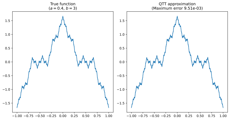
When we compare this with the true Weierstrass function, we get an encouraging figure.

Error Analysis

Let us assume that \(Q\) is an exact representation of \(f\) on the grid with \(b^\ell\) points. We will also assume that \(f\) is differentiable. Since \(f\) is periodic, its derivative is bounded; say that \(\vert f’(x) \vert <D\). In a slight abuse of notation, write \(Q(x)\) to indicate the value of the QTT \(Q\) at the point \(x\), as long as \(x\) is a point where the QTT can be evaluated exactly. Then our error is \[\max_{b^Lx \in \mathbb{Z}} \left| W_{a,b}[f](x) - \sum_{n=0}^{L-1}E_{n,L-\ell-n}[Q](x)-\frac{a^L}{1-a}g(x) \right|.\] This is bounded above by \[\begin{align}\max & \left( \sum_{n=0}^{L-\ell-1} a^n \left| f(b^n x) - E_{n,L-\ell-n}[Q](x)\right| \right. \\ & \left.+ \sum_{n=L-\ell}^{L-1}a^n \left| f(b^n x) - E_{n,L-\ell-n}[Q](x)\right| \right. \\ & \left. + \left| \left[\sum_{n=L}^\infty a^n f(b^n x)\right] - \frac{a^L}{1-a}g(x)\right|\right).\end{align}\] Since \(Q\) is an exact representation of \(f\), the second term is zero; since our representation of \(g\) is exact as well, so is the third term. The remaining error is \[\max \sum_{n=0}^{L-\ell-1} a^n \left| f(b^n x) - E_{n,L-\ell-n}[Q](x)\right|.\]

To bound this, we note that \(f(b^n x)\) agrees with \(E_{n,L-\ell-n}[Q](x)\) on a grid of \(b^{\ell + n}\) elements. Since \(E_{n,L-\ell-n}[Q](x)\) is otherwise constant, and \(\vert f’(x) \vert <D\), \[a^n \left| f(b^n x) - E_{n,L-\ell-n}[Q](x)\right| < \frac{a^n}{b^{\ell+n}}D.\] Then the total error is at most \[\sum_{n=0}^{L-\ell-1}\frac{a^n}{b^{\ell+n}}D = \frac{b^{1-\ell}-b^{-L}a^{L-\ell}}{b-a} < b^{-\ell}.\]

The rank of our final QTT is bounded by \(R := \ell r + (L - \ell) + 2\), since every bond is the sum of \(\ell\) bonds of rank at most \(r\), \(L-\ell\) of rank \(1\), and one of rank \(2\). Rearranging, \(\ell = \frac{R-L-2}{r-1}\). Assuming that \(r\) is much greater than \(L\), \(\ell \approx R/r\). Therefore, in the large-\(r\) regime, the error of our Weierstrass QTT decays approximately as \(b^{-R/r}\). To accomplish this, it requires \(O(LR^2b)\) storage.