Paul Michael Kielstra

Introduction: QTTs, Kernels, Convolution, and Subtraction

I’m going to assume that you basically know what a quantized tensor train (QTT) is. If you don’t know what a tensor train is, you can read about them here; if you don’t know what a quantized tensor train is, you can read about them here. The gist is that we compress a function \(f\) into an \(n\)-tensor \(T\) such that \(T_{i_1i_2\dots i_n} = f(0.i_1i_2\dots i_n)\). In general, the decimal expansion is done in binary, so \(i_j \in {0, 1}\). For example, \(T_{1,0,0,\dots,0}=f(1/2)\).

\(T\) on its own is going to be very large, but, if \(f\) is periodic or nearly so, or Lipschitz continuous with a small Lipschitz constant, or just generally “nice,” we can write \(T\) as a tensor train with low internal bond dimension. There are various ways to do this, and I’ll take it as read that you’ve found one you like. That’s the setting for what’s to come: we have a function \(f\), compressed into a tensor train with cores \(T^1, \dots, T^n\). We also have a point \(x \in (0, 1)\) at which we want to evaluate \(f\), and we write the binary expansion as \(x=0.i_1i_2\dots i_n\).

We often want to compute functions of the form \(k(x, y) = f(x - y)\) . These can be used in kernel methods, or to calculate convolutions. Given how much this relies on \(f\), we might expect that there is some way to transform a QTT for \(f\) into one for \(k\) without doing much extra work. This does in fact turn out to be the case, but, to understand how, we’re going to have to take a couple of detours.

I heard these ideas from Michael Lindsey, who told me that they were more or less unattributed folk wisdom.

Part 0: The Care and Feeding of QTTs

A QTT looks something like this:

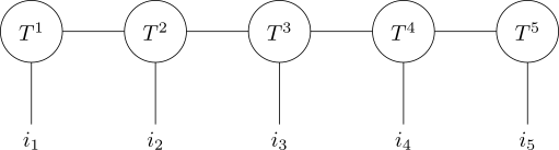
The dimensions of the internal bonds can vary, but we assume that they’re low enough to make the compression worthwhile. The dimension of each dangling edge is exactly \(2\).

Intuitively, we imagine each dangling edge as a “socket” into which we can put a single binary bit of information. Combine all those bits together into a binary expansion and you get a number out. However, that’s not normally something you want to do with QTTs – or with any tensor network, really. In general, we prefer contracting tensor networks as tensor networks to pulling out individual data points from them.

To explain why, think about how we might extract, say, \(T_{0,1,1,0,1}\) from our original tensor \(T\). We would go dimension by dimension, choosing either the first or the second element, and inductively working our way down until we reached a single scalar value. This is easy to do when you’ve got \(T\) stored in memory as an array – but we very explicitly do not have \(T\) stored in memory as an array. That’s the point of the tensor train. If we’re “doing this right,” then \(T\) should be far too large to ever form entirely. So we’re going to have to restrict ourselves to operations that we can carry out on small chunks of the tensor train, locally, and contraction is the standard and most versatile one.

So we can’t just pick an individual element along each dangling edge. What if we could come up with a list of tensors to which we could link those edges, so that when we carried out the entire contraction, which we could do part by part without using too much memory, we’d get the answer we wanted?

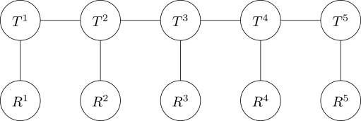
These tensors \(R^k\) aren’t actually that hard to build. They each have one edge, so they’re one-dimensional. We just set \(R^k_j = 1\) when \(j=i_k\) and \(0\) otherwise. (Remember that \(i_k\) is the \(k\)-th element of our decimal expansion.) That way, when we contract, we’re guaranteed to zero out every element of \(T^k\) which doesn’t correspond to the correct choice of digit, and leave those that do unchanged.

To see why this works, let’s go back to thinking of our uncompressed giant tensor \(T\). Then, the equivalent of the contraction that we’ve just done on our tensor train would be \(\sum_{j_1, j_2, \dots, j_n} T_{j_1j_2\dots j_n} R^1_{j_1}R^2_{j_2}\cdots R^n_{j_n}\). The only term where at least one of the \(R\)s isn’t \(0\) is when \(j_1=i_1\), \(j_2=i_2\), and so on. All other terms disappear, and we’re left with exactly \(T_{i_1i_2\dots i_n}\) as expected.

Rather than restrict ourselves to carving up tensors by hand, we can use these “one-hot encoded” auxiliary tensors and reduce to doing a tensor network contraction. This is exciting if we just have a black-box contraction algorithm; even more excitingly, though, it lets us think of tensors not just as overgrown matrices, but also as functions in their own right. We can think of \(R^k\) as the tensor which “outputs \(i_k\)” – whenever we attach it to a dangling edge, it’s as if we artificially restricted that edge to the single value \(i_k\).

Part 1: “Function Tensors” and Addition

Tensors can have “inputs” as well as “outputs.” We can associate the function \(b: \mathbb{N} \rightarrow \mathbb{N}\) with the tensor \(B_{xy}\), where \(B_{xy}=1\) if and only if \(b(x)=y\). (As usual, \(B\) is \(0\) otherwise.) Now, if we attach \(B\) to each leg of a quantized tensor train for a function \(f\), thus:

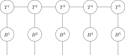
then we get, for free, a quantized tensor train for the function of \(x\) represented by writing \(x\) as a binary expansion, applying \(b\) to each bit, turning the result back into a real number, and applying \(f\).

For more on formulating tensors as functions, see Peng, Gray, and Chan, 2023. Their approach is slightly different to this one but they’re doing the same kind of thing.

There are obviously lots of things we can do with our “augmented tensor trains” right away. If we already have a binary expansion for \(x \in (0, 1)\), then we can get a binary expansion for \(1 - x\) just by flipping each bit. (Remember this. It’ll be important later.) So now we’ve managed to reflect \(f\) around \(1\). We can do more complicated bit masking, bit flipping, bitwise XOR with a fixed known cyphertext we’re trying to crack, anything.

That said, there are quite a few operations which are not simply bitwise. The one we really want to do, that will allow us to get our function \(k(x, y)=f(x-y)\) as above, is subtraction, but that’s going to be trickier, so let’s start with addition. We’ll try to build a tensor train for \(x, y \mapsto f(x + y)\).

Even before we put our tensors together, this is going to have a caveat. If we take \(x, y \in (0, 1)\), as we would like to do, then \(x + y\) is not always in \((0, 1)\). It’s in \((0, 2)\). So, rather than having binary expansions that look like \(0.i_1i_2\dots i_n\), we’ll have binary expansions that look like \(i_1.i_2i_3\dots i_{n+1}\). Note the extra digit at the front. This is why it’s so useful to use binary expansions, instead of, say, hexadecimal: they handle this kind of doubling of the state space really elegantly.

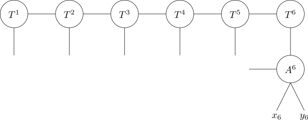
Now, let’s write \(x=0.x_2x_3 \dots x_{n+1}\) and \(y=0.y_2y_3\dots y_{n+1}\). (I’m removing \(x_1\) and \(y_1\) to keep the notification consistent.) When we want to add two decimal expansions, as we learned in grade school, we start from the far right, so let’s tack on a tensor \(A^{n+1}_{xyrc}\) to the far right of the tensor train. It’s going to have four edges. The \(x\) edge and \(y\) edge are going to take \(x_{n+1}\) and \(y_{n+1}\) as input, the \(r\) edge (r for result) is going to output the right-hand digit of \(x_{n+1}+y_{n+1}\), and the \(c\) edge is going to output the carry bit.

In tensor terms, that means that \(A^{n+1}_{xyrc}=1\) at exactly these values:

\(x\)	\(y\)	\(r\)	\(c\)
0	0	0	0
0	1	1	0
1	0	1	0
1	1	0	1

Now we connect the \(r\) edge to the \(i_{n+1}\) edge on our original tensor train, and leave the \(x\) and \(y\) edges dangling. The \(c\) edge, which here points to the left, is also left dangling for now:

The tensors attached to the other dangling edges of the original QTT are going to be slightly more complicated. They have to deal with everything that \(A^{n+1}\) has to deal with, and an incoming carry bit on top of that. Luckily, they’re all going to be identical. For \(k \in {2, \dots, n}\), define \(A^k_{xyc’rc}\) to be the function where \(r\) is the result and \(c\) the carry bit from adding \(x\), \(y\), and the incoming carry bit \(c’\). Again, we can write out the list of points where \(A^k_{xyc’rc}=1\):

\(x\)	\(y\)	\(c’\)	\(r\)	\(c\)
0	0	0	0	0
0	0	1	1	0
0	1	0	1	0
0	1	1	0	1
1	0	0	1	0
1	0	1	0	1
1	1	0	0	1
1	1	1	1	1

Then we just attach copies of this together, connecting each \(c’\) edge to the previous tensor’s \(c\) edge. The last one gets attached to not one, but two tensors in the original tensor train, since it’s got nowhere else to put its carry bit:

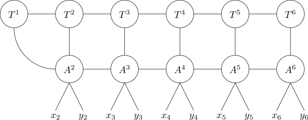
This is technically not a tensor train any more, but it can be turned into one with just \(O(N)\) contractions along edges with mostly very low dimension. We’ve as good as got ourselves a QTT for \(x, y \mapsto f(x+y)\). In particular, every edge of each \(A\) tensor has dimension exactly \(2\), so the interior bond dimension of our tensor train has only doubled (and might increase even less than that if we include another compression step)!

Part 2: Subtraction (Finally)

Subtracting things is much harder than adding them, because sometimes \(y > x\), and then \(x - y\) is negative. The remainder of our task is, more or less, to come up with a way to get around this. We’ll begin by noting that \(x - y = x + (1 - y) - 1\), which seems not to help us very much until we realize that, for \(y \in (0, 1)\), \(1-y \in (0, 1)\) as well – and, as I mentioned earlier, we can get \(1-y\) by flipping the bits for \(y\). So define the bit-flip tensor \(B_{pq}=1\) when \(p \neq q\), and attach one of those to each \(y\) leg of the QTT-like construction from the previous part, thus:

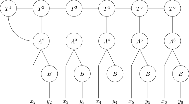
We now have (something very close to) a QTT for the function \(x, y \mapsto f(x - y + 1)\). Now, at this point, we could in theory play around with the individual bits to subtract off the constant. That, however, would require another set of tensors with some horizontal communication between them for borrowing, which would increase the bond dimension of the overall QTT. What’s much easier is to simply go back in time and decide that, when we did the original compression for the function \(f(z)\), we did not actually compress \(f(z)\), but rather \(f(z-1)\).

This isn’t such an unreasonable thing. If \(f\) compresses nicely on \((-1, 1)\), then \(f(z-1)\) compresses nicely on \((0, 2)\). And, by using a constant tensor to force the first bit of the binary expansion to be \(1\), we can recover \(f(z)\) from \(f(z-1)\) if we really want to. But that’s beside the point. The point is that, if \(f(z)\) has a low-rank QTT representation, then so must \(k(x, y)=f(x-y)\), and, moreover, we can write code that finds it in not much more time than it takes to find the QTT representation for \(f\).

Three possible optimizations stand out for a practical implementation:

• Often, we are interested not just in \(f(x-y)\) but in \(f(|x-y|)\). This could be used to cut the area over which \(f\) must be sampled in half.

• We can contract the \(A\) and \(B\) tensors together by hand and determine a new, combined tensor, which we could hardcode into our algorithm instead of using \(A\) and \(B\) directly.

• We only need to store \(O(1)\) \(A\) and \(B\) tensors (or combined \(AB\) tensors) since most of them are identical to each other.

A basic code for this is conceptually simple, if you use a decent tensor network library. I would encourage you to write your own.